
This is a guest entry written by Rolf Rolles from Mobius Strip Reverse Engineering. His views and opinions are his own, and not those of Hex-Rays. Any technical or maintenance issues regarding the code herein should be directed to him.
In this entry, we’ll investigate an in-the-wild malware sample that was compiled by an obfuscating compiler to hinder analysis. We begin by examining its obfuscation techniques and formulating strategies for removing them. Following a brief detour into the Hex-Rays CTREE API, we find that the newly-released microcode API is more powerful and flexible for our task. We give an overview of the microcode API, and then we write a Hex-Rays plugin to automatically remove the obfuscation and present the user with a clean decompilation.
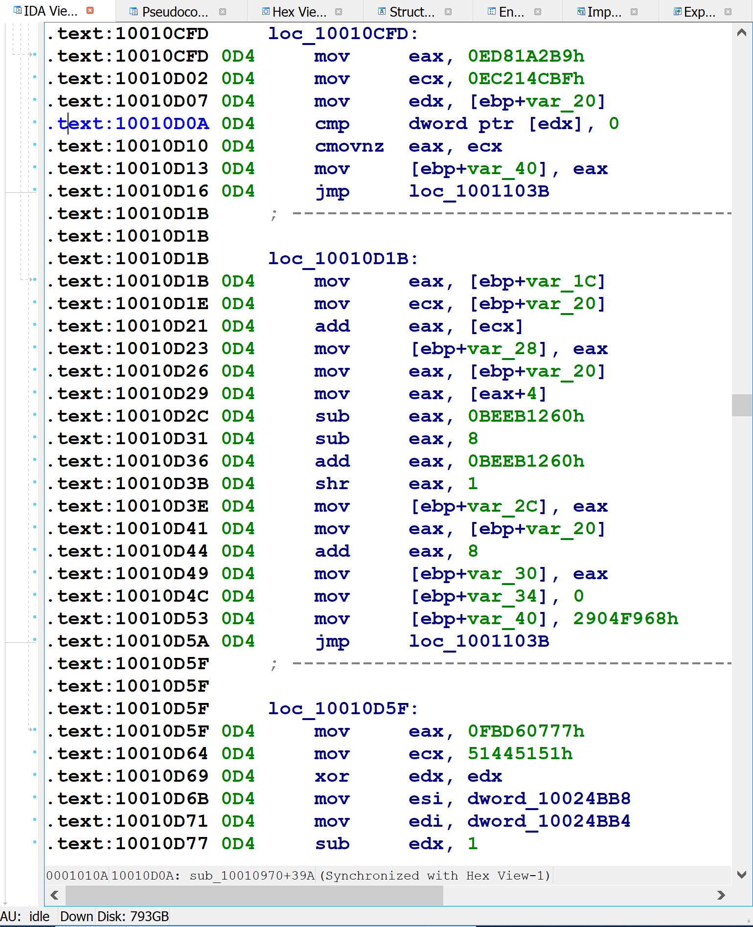
The plugin is open source and weighs in at roughly 4KLOC of heavily-commented C++. Additionally, we are also releasing a helpful plugin for aspiring microcode plugin developers called the Microcode Explorer, which will also be distributed with the Hex-Rays SDK in subsequent releases. In brief, for the sample we’ll explore in this entry, its assembly language code looks like this:
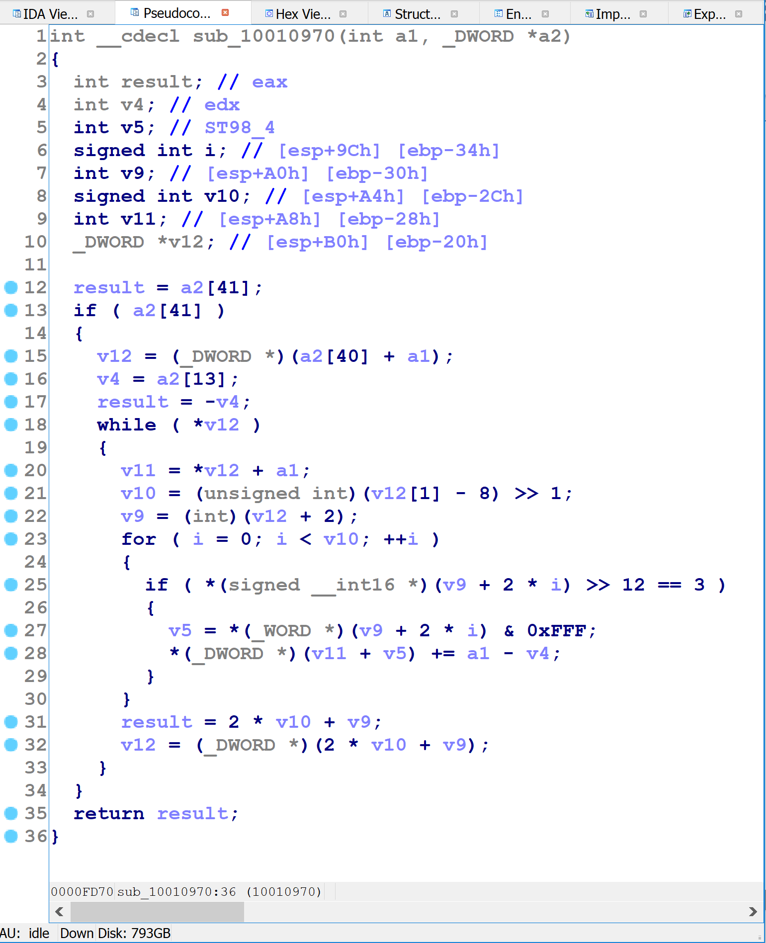
That function’s Hex-Rays decompilation looks like this:
Once our deobfuscation plugin is installed, it will automatically rewrite the decompilation to look like this:
Initial Investigation
The sample we’ll be examining was given to me by a student in my SMT-based binary analysis class. The binary looks clean at first. IDA’s navigation bar doesn’t immediately indicate tell-tale signs of obfuscation:

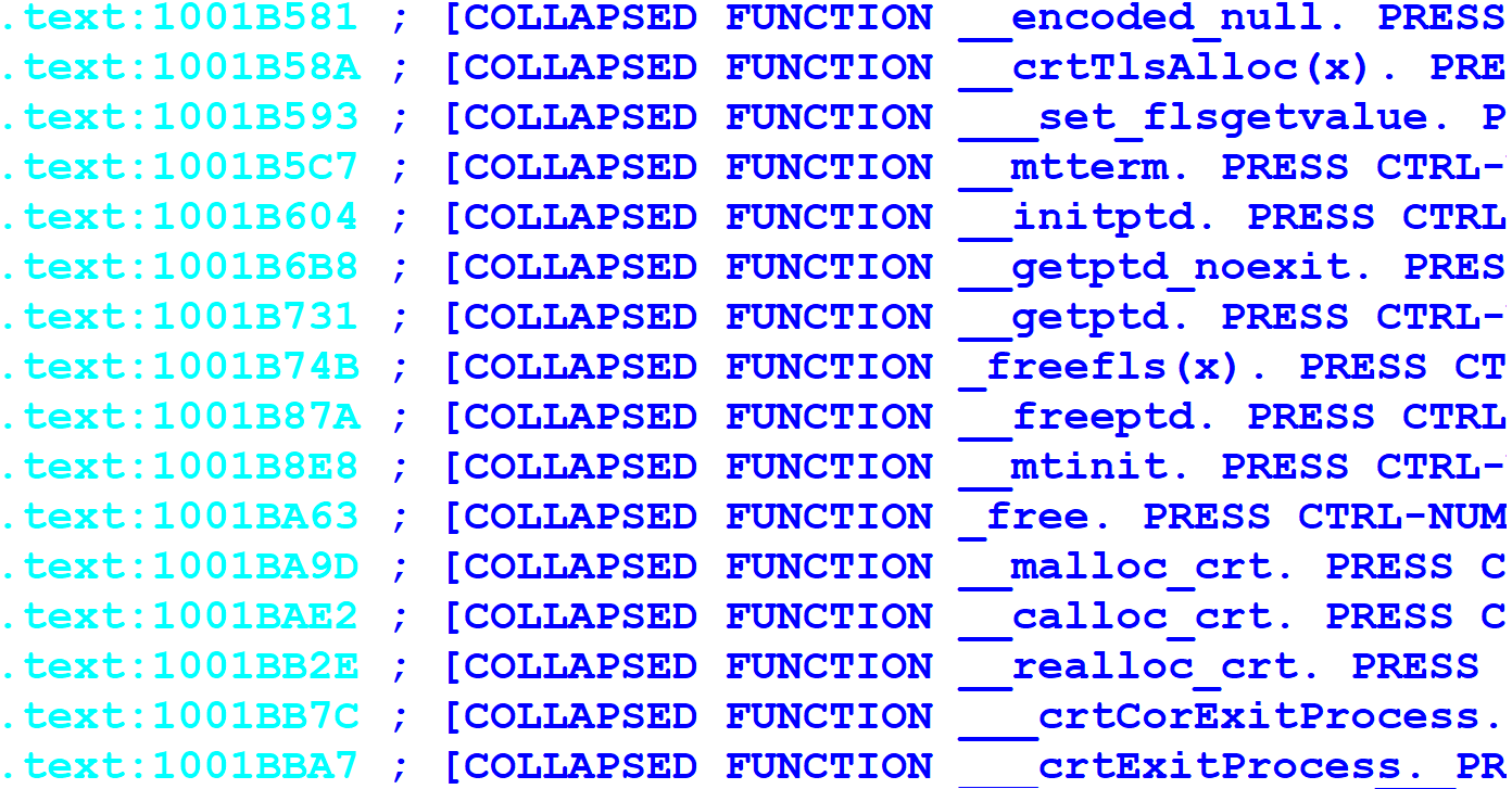
The binary is statically linked with the ordinary Microsoft Visual C runtime, indicating that it was compiled with Visual Studio:
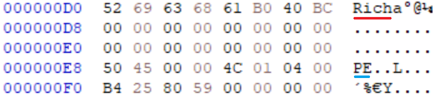
And finally, the binary has a RICH header, indicating that it was linked with the Microsoft Linker:
Thus far, the binary seems normal. However, nearly any function’s assembly and decompilation listings immediately tells a different tale, as shown in the figures at the top of this entry. We can see constants with high entropy, redundant computations that an ordinary compiler optimization would have removed, and an unusual control flow structure.
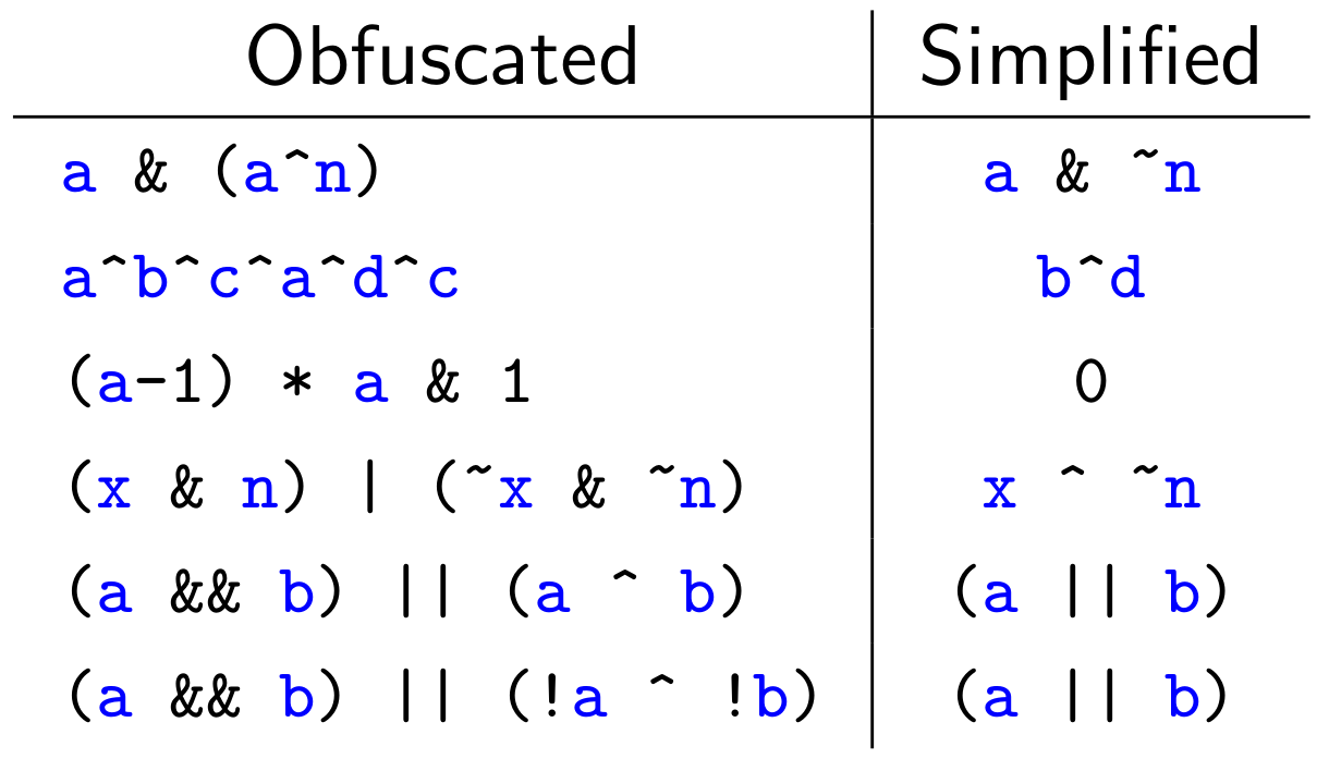
Pattern-Based Obfuscation
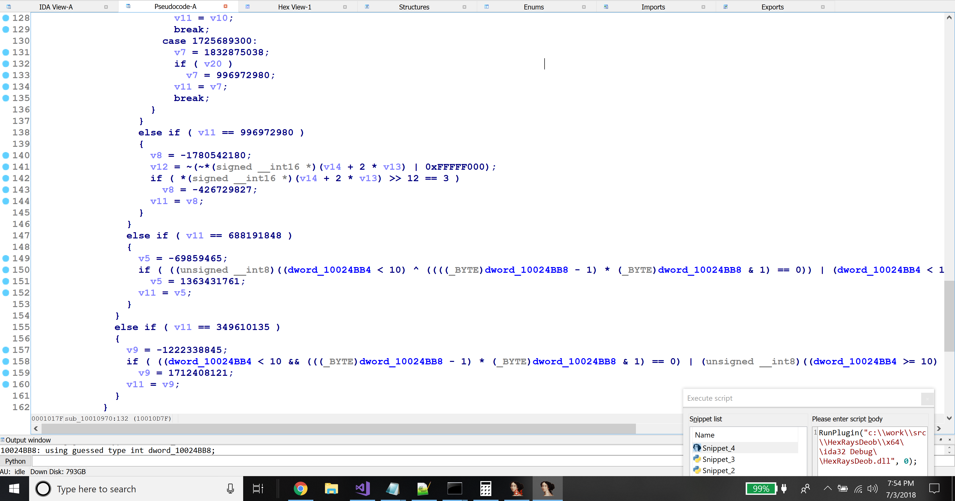
In the decompilation listing, we see repeated patterns:
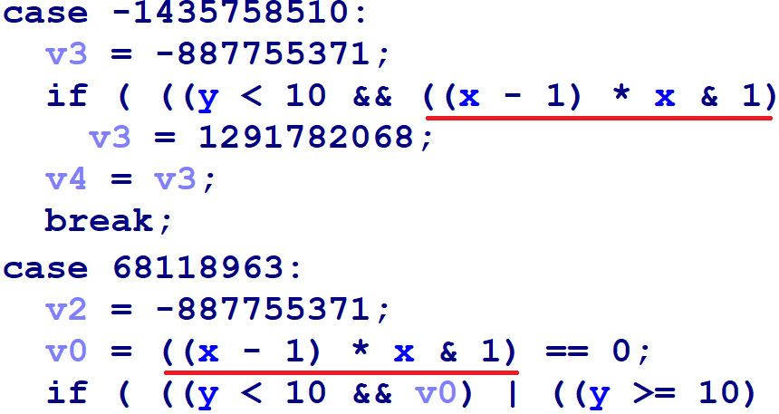
The underlined terms are identical. With a little thought, we can determine that the underlined sequence always evaluates to 0 at run-time, because:
xis either even or odd, andx-1has the opposite parity- An even number times an odd number is always even
- Even numbers have their lowest bit clear
- Thus, AND by
1produces the value0
That the same pattern appears repeatedly is an indication that the obfuscating compiler has a repertoire of patterns that it introduces into the code prior to compilation.
Opaque Predicates
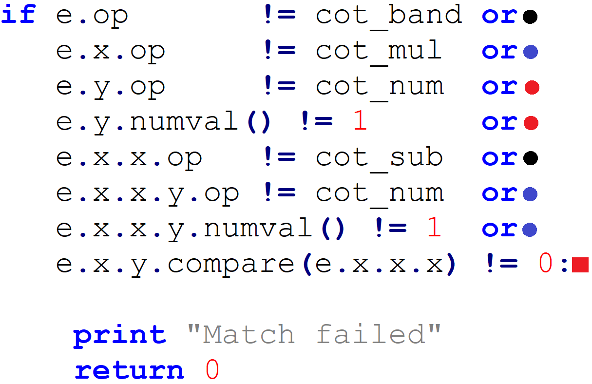
Another note about the previous figure is that the topmost occurrence of the x*(x-1) & 1 pattern is
inside of an if-statement with an AND-compound conditional. Given that this expression always evaluates
to zero, the AND-compound will fail and the body of the if-statement will never execute. This is a form of
obfuscation
known as opaque predicates: conditional branches that in fact are not conditional, but can only evaluate one way or
the
other at runtime.
Control-Flow Flattening
The obfuscated functions exhibit unusual control flow. Each contains a switch statement in a loop
(though
the “switch statement” is compiled via binary search instead of with
a table). This is evidence of a well-known form of obfuscation called “control flow flattening”. In brief, it works
as
follows:
- Assign a number to each basic block.
- The obfuscator introduces a block number variable, indicating which block should execute.
- Each block, instead of transferring control to a successor with a branch instruction as usual, updates the block number variable to its chosen successor.
- The ordinary control flow is replaced with a switch statement over the block number variable, wrapped inside of a loop.
The following animation illustrates the control-flow flattening process:
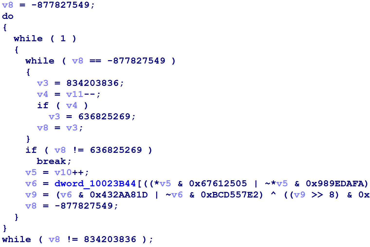
Here’s the assembly language implementation of control flow flattening switch for a small function.
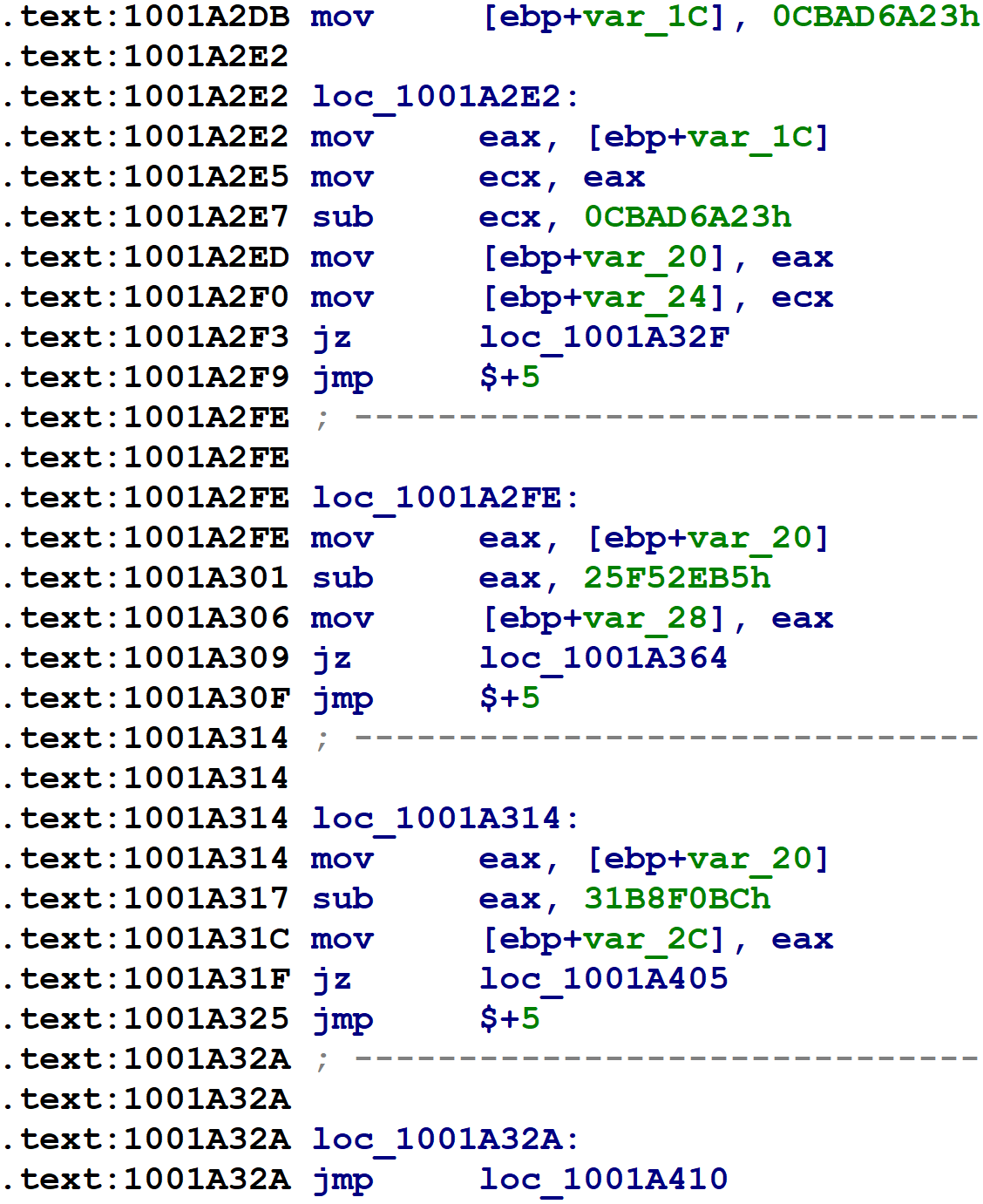
On the first line, var_1C — the block number variable mentioned above — is initialized to some
random-looking number. Immediately following that is a series of comparisons of var_1C against other
random-looking numbers. (var_1C is copied into var_20, and var_20 is used
for comparisons after the first.)
The targets of these equality comparisons are the original function’s basic blocks. Each one updates
var_1C to indicate which block should execute next, before branching back to the code just shown, which
will then perform the equality comparisons and select the corresponding block to execute. For blocks with one
successor,
the obfuscator simply assigns var_1C to a constant value, as in the following figure.
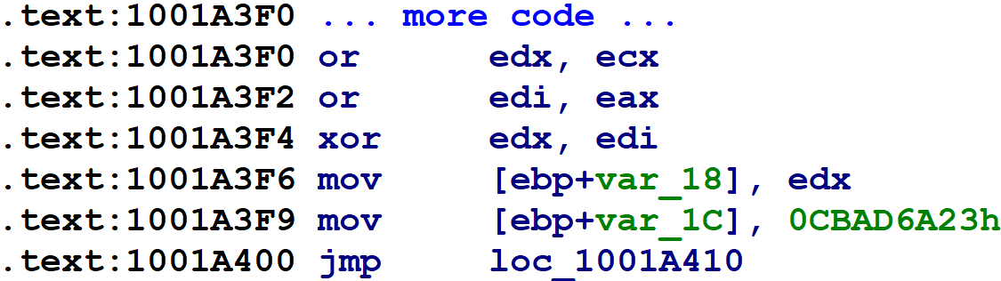
For blocks with two possible successors (such as if-statements), the obfuscator introduces x86 CMOV
instructions to set var_1C to one of two possible values, as shown below:
Graphically, each function looks like this:
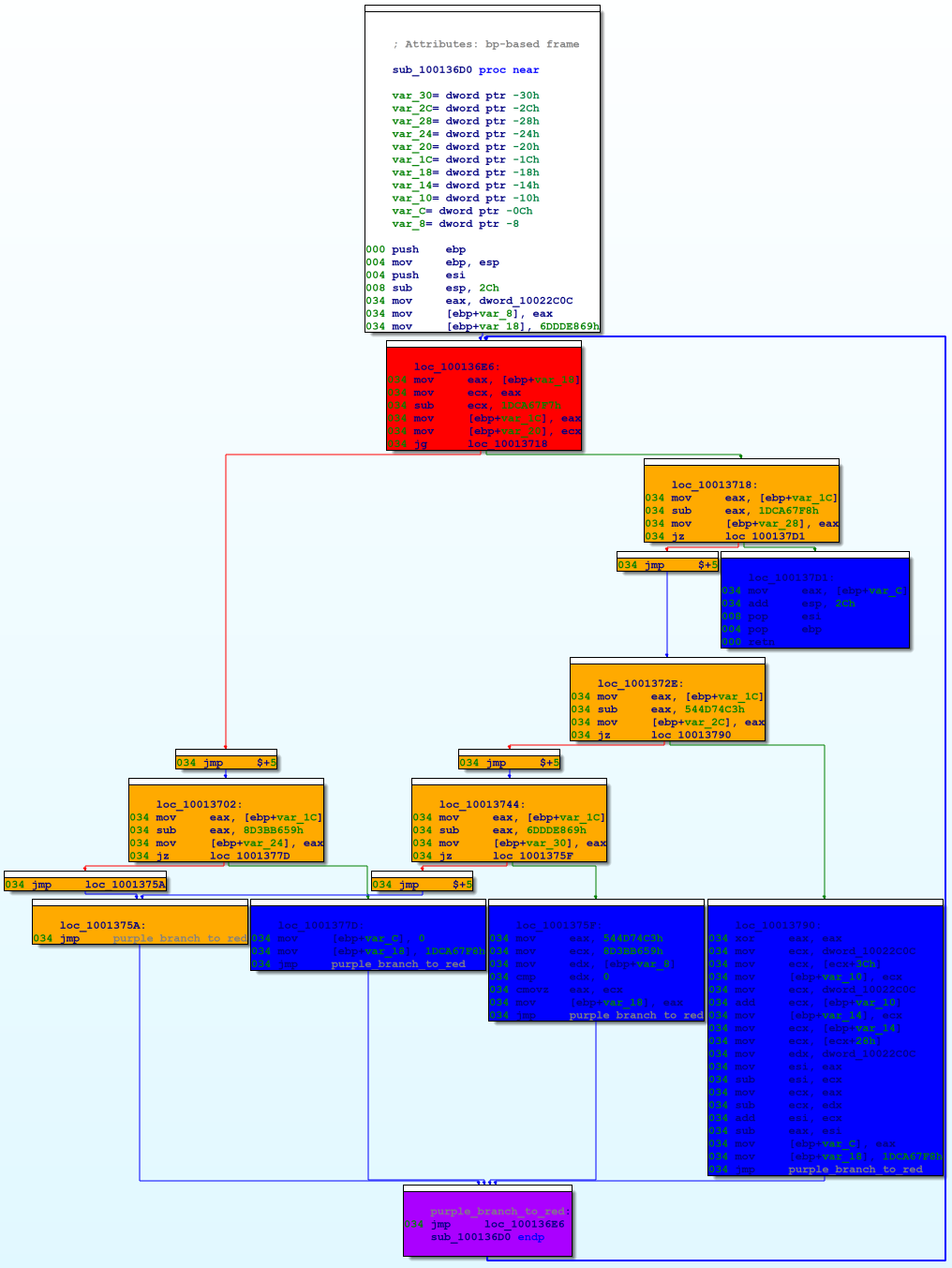
In the figure above, the red and orange nodes are the switch-as-binary-search implementation. The blue nodes are the original basic blocks from the function (subject to further obfuscation). The purple node at the bottom is the loop back to the beginning of the switch-as-binary-search construct (the red node).
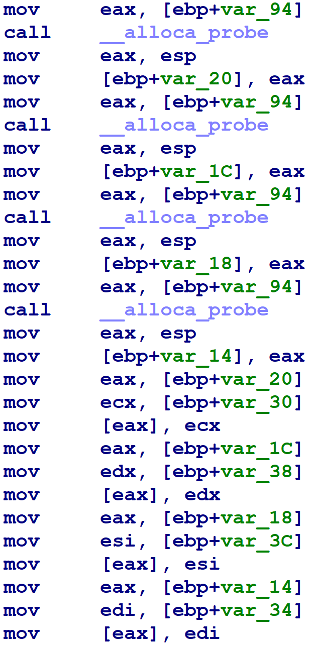
Odd Stack Manipulations
Finally, we can also see that the obfuscator manipulates the stack pointer in unusual ways. Particularly, it uses
__alloca_probe to reserve stack space for function arguments and local variables, where a normal
compiler
would, respectively, use the push instruction and reserve space for all local variables at once in the
prologue.
IDA has built-in heuristics to determine the numeric argument to __alloca_probe and track the effects of
these calls upon the stack pointer. However, the output of the obfuscator leaves IDA unable to determine the numeric
argument, so IDA cannot properly track the stack pointer.
Aside: Where did this Binary Come From?
I am not entirely sure how this binary was produced. Obfuscator-LLVM
also uses pattern-based obfuscation and control flow flattening, but Obfuscator-LLVM has different patterns than
this
sample, and there are some superficial differences with how control flow flattening is implemented. Also,
Obfuscator-LLVM does not generate opaque predicates, nor the alloca-related obfuscation. And, needless
to
say, the fact that the binary includes the Microsoft CRT and a RICH header is also puzzling. If you have any further
information about this binary, please contact me.
Update: following discussions on twitter with an Obfuscator-LLVM developer and another knowledgeable individual, in fact, the obfuscating compiler in question is Obfuscator-LLVM, which has been integrated with the Microsoft Visual Studio toolchain. The paragraph above falsely stated that Obfuscator-LLVM used different patterns and did not insert opaque predicates. The author regrets these errors. In theory, the plugin we develop in this entry might work for other binaries produced by the same compilation process, or even for Obfuscator-LLVM in general, but this theory has not been tested and no guarantees are offered.
Plan of Attack
Now that we’ve seen the obfuscation techniques, let’s break them.
A maxim I’ve learned doing deobfuscation is that the best results come from working at the same level of abstraction that the obfuscator used. For obfuscators that work on the assembly-language level, historically my best results have come in using techniques that represent the obfuscated code in terms of assembly language. For obfuscators that work at the source- or compiler internal-level, my best results have come from using a decompiled representation. So, for this obfuscator, a Hex-Rays plugin seemed among our best options.
The investigation above illuminated four obfuscation techniques for us to contend with:
- Pattern-based obfuscation
- Opaque predicates
- Alloca-related stack manipulation
- Control flow flattening
The first two techniques are implemented via pattern substitutions inside of the obfuscating compiler. Pattern-based deobfuscation techniques, for all their downsides, tend to work well when the obfuscator itself employed a repertoire of patterns — especially a limited one — as seems to be the case here. So, we will attack these via pattern matching and replacement.
The alloca-related stack manipulation is the simplest technique to bypass. The obfuscator’s non-standard
constructs have thwarted IDA’s ordinary analysis surrounding calls to __alloca_probe, and hence the
obfuscation prevented IDA from properly accounting for the stack differentials induced by these calls. To break this, we
will let Hex-Rays do most of the work for us. For every function that calls __alloca_probe, we will use
the API to decompile it, and then at every call site to __alloca_probe, we will extract the numeric value
of its sole argument. Finally, we will use this information to create proper stack displacements within the disassembly
listing. The code for this is very straightforward.
As for control flow flattening, this is the most complicated of the transformations above. We’ll get back to it later.
First Approach: Using the CTREE API
I began my deobfuscation by examining the decompilation of the obfuscated functions and cataloging the obfuscated patterns therein. The following is a partial listing:
Though I later switched to the Hex-Rays microcode API, I started with the CTREE API, the one that has been available since the first releases of the Hex-Rays SDK. It is overall simpler than the microcode API, and has IDAPython bindings where the microcode API currently does not.
The CTREE API provides a data structure representation of the decompiled code, from which the decompilation listing that
is presented to the user is generated. Thus, there is a direct, one-to-one correspondence between the decompilation
listing and the CTREE representation. For example, an if-statement in the decompilation listing corresponds to a CTREE
data structure of type cif_t, which contains a pointer to a CTREE data structure of type
cexpr_t representing the if-statement’s conditional expression, as well as a pointer to a
CTREE data structure of type cinsn_t representing the body of the if-statement.
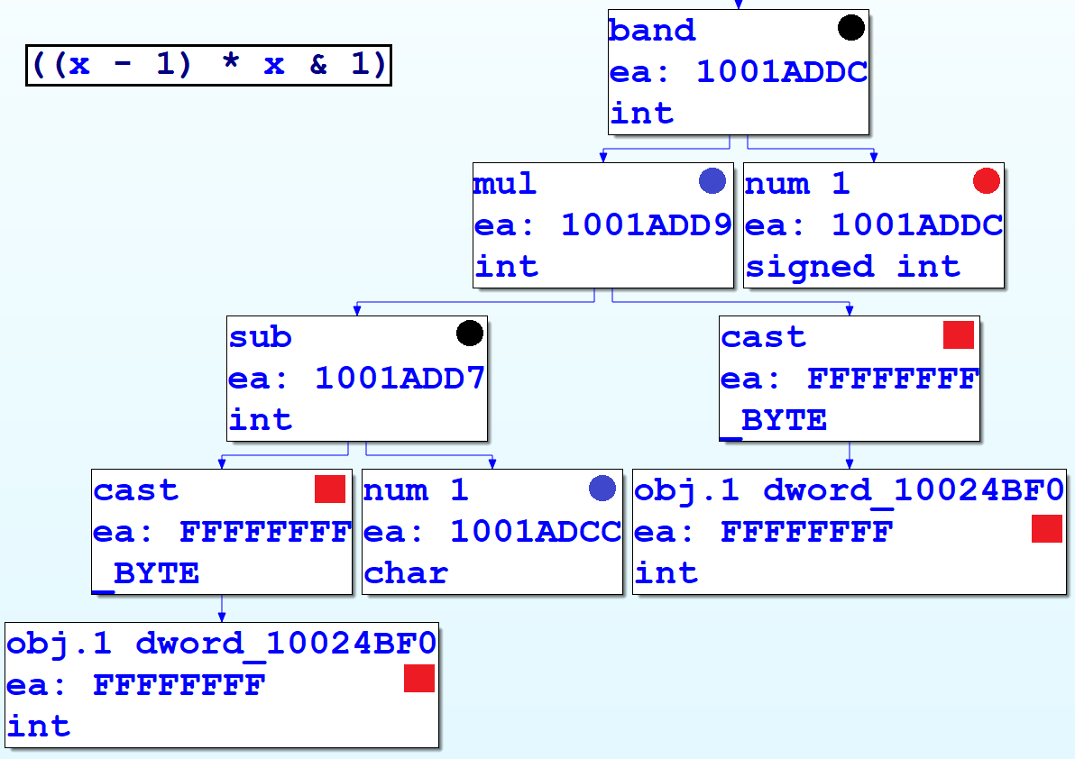
We will need to know how our patterns are represented in terms of CTREE data structures. To assist us, the VDS5 sample plugin from the Hex-Rays SDK helpfully displays the graph of a function’s CTREE data structures. (The third-party plugin HexRaysCodeXplorer implements this functionality in terms of IDA’s built-in graphing capabilities, whereas the VDS5 sample uses the external WinGraph viewer.) The following figure shows decompilation output (in the top left) and its corresponding CTREE representation in graphical form. Hopefully, the parallels between them are clear.
To implement our pattern-based deobfuscation rules, we simply need to write functions to locate instances within the
function’s CTREE of the data types associated with the obfuscated patterns, and replace them with CTREE versions of
their deobfuscated equivalents. For example, to match the (x-1) * x & 1 pattern we saw before, we
determine the CTREE representation and write an if-statement that matches it, as follows:
In practice, these rules should be written more generically when possible. I.e., multiplication and bitwise AND are commutative; the pattern matching code should be able to account for this, and match terms with the operands swapped. Also, see the open-source project HRAST for an IDAPython framework that offers a less cumbersome approach to pattern-matching and replacement.)
The only point of subtlety in replacing obfuscated CTREE elements with deobfuscated equivalents is that each CTREE expression has associated type information, and we must carefully ensure that our replacements are of the proper type. The easiest solution is simply to copy the type information from the CTREE expression we’re replacing.
First Major CTREE Issue: Compiler Optimizations
Cataloging the patterns and writing match and replace functions for them was straightforward. However, after having done so, the decompilation showed obvious opportunities for improvement by application of standard compiler optimizations, as shown in the following animation.
This perplexed me at first. I knew that Hex-Rays already implemented these compiler optimizations, so I was confused that they weren’t being applied in this situation. Igor Skochinsky suggested that, while Hex-Rays does indeed implement these optimizations, that they take place during the microcode phase of decompilation, and that these optimizations don’t happen anymore once the CTREE representation has been generated. Thus, I would either have to port my plugin to the microcode world, or write these optimizations myself on the CTREE level. I set the issue aside for the time being and continued with the other parts of the project.
Control Flow Unflattening via the CTREE API
Next, I began working on the control flow unflattening portion. I envisioned this taking place in three stages. My final solution included none of these steps, so I won’t devote a lot of print space to my early plan. But, I’ll discuss the original idea, and the issues that lead me to my final solution.
- Starting from the switch-as-binary-search implementation, rebuild an actual
switchstatement (rather than a mess of nestedifandgotostatements). - Examine how each switch case updates the block number variable to recover the original control flow graph. I.e., each update to the block number variable corresponds to an edge from one block to its numbered target.
- Given the control flow graph, reconstruct high-level control flow structures such as loops,
if/elsestatements,break,continue,return, and so on.
I began by writing a CTREE-based component to reconstruct switch statements from obfuscated functions. The basic idea — inspired by the assembly language implementation — is to identify the variable that represents the block number to execute, find equality comparisons of this variable against constant numbers, and extract these numbers (these are the case labels) as well the address of the code that executes if the comparison matches (these are the bodies of the case statements).
This proved more difficult than I expected. Although the assembly language implementations had a predictable structure, Hex-Rays had applied transformations to the high-level control flow which made it difficult to extract the information I was after, as we can see in the following figure.
We see above the introduction of a strange while loop in the inner switch, and the final
if-statement has been inverted to a != conditional rather than a ==
conditional, which might seem a more logical translation of the assembly code. The example above doesn’t show it, but
sometimes Hex-Rays rebuilds small switch statements that cover portions of the larger
switch. Thus, our switch reconstruction logic must take into account that these
transformations might have taken place.
For ordinary decompilation tasks, these transformations would have been valuable improvements to the output; but in my unusual situation, it meant my switch recovery algorithm was basically fighting against these transformations. My first attempt at rebuilding switches had a lot of cumbersome corner cases, and overall did not work very well.
Control Flow Reconstruction
Still, I pressed on. I started thinking about how to rebuild high-level control flow structure (if
statements, while loops, returns, etc.) from the recovered control flow graph. While it
seemed like a fun challenge, I quickly realized that Hex-Rays obviously already includes this functionality. Could I
re-use Hex-Rays’ existing algorithms to do that?
Another conversation with Igor lead to a similar answer as before: in order to take advantage of Hex-Rays’ built-in control flow structuring algorithms, I would need to operate at the microcode level instead of the CTREE level. At this point, all of my issues seemed to be pointing me toward the newly-available microcode API. I bit the bullet and started over with the project using the microcode API.
Overview of the Hex-Rays Microcode API
My first order of business was to read the SDK’s hexrays.hpp, which now includes the microcode API. I’ll
summarize some of my findings here; I have provided some more, optional information in an appendix.
At Igor’s suggestion, I compiled the VDS9 plugin included with the Hex-Rays SDK. This plugin demonstrates how to
generate microcode for a given function (using the gen_microcode() API) and print it to the output window
(using mbl_array_t::print()).
Microcode API Data Structures
For my purposes, the most important things to understand about the microcode API were four key data structures:
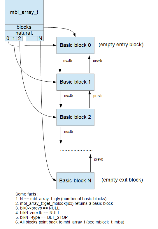
minsn_t, microcode instructions.mop_t, operands for microcode instructions.mbl_array_t, which contains the graph for the microcode function.mblock_t, the basic blocks within the microcode graph, which contain the instructions, and the edges between the blocks.
For the first two points, Ilfak has given an overview presentation about the microcode instruction set. For the second two points, he has published a blog entry showing graphically how all of these data structures relate to one another. Aspiring microcode API plugin developers would do well to read those entries; the latter includes many nice figures such as this one:
Microcode Maturity
As Hex-Rays internally optimizes and transforms the microcode, it moves through so-called “maturity phases”, indicated
by an enumerated element of type mba_maturity_t. For example, immediately after generation, the microcode
is said to be at maturity MMAT_GENERATED. After local optimizations have been performed, the microcode
moves to maturity MMAT_LOCOPT. After performing analysis of function calls (such as deciding which pushes
onto the stack correspond to which called function), the microcode moves to maturity MMAT_CALLS. When
generating microcode via the gen_microcode() API, the user can specify the desired maturity level to
which the microcode should be optimized.
The Microcode Explorer Plugin
Examining the microcode at various levels of maturity is an informative and impressive undertaking that I recommend for all would-be microcode API plugin developers. It sheds light on which transformations take place in which order, and the textual output is easy to comprehend. At the start of this project, I spent a good bit of time reading through microcode dumps at various levels of maturity.
Though the microcode dump output is very nice and easy to read, its output does not show the low-level details of how
the microcode instructions and operands are represented — which is critical information for writing microcode plugins.
As such, to understand the low-level representation, I wrote functions to dump minsn_t instructions and
mop_t operands in textual form.
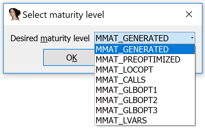
For the benefit of would-be microcode plugin developers, I created a plugin I call the Microcode Explorer. With your cursor within a function, run the plugin. It will ask you to select a decompiler maturity level:
Once the user makes a selection, the plugin shows a custom viewer in IDA with the microcode dump at the selected maturity level.
The microcode dump is mostly non-interactive, but it does offer the user two additional features. First, pressing
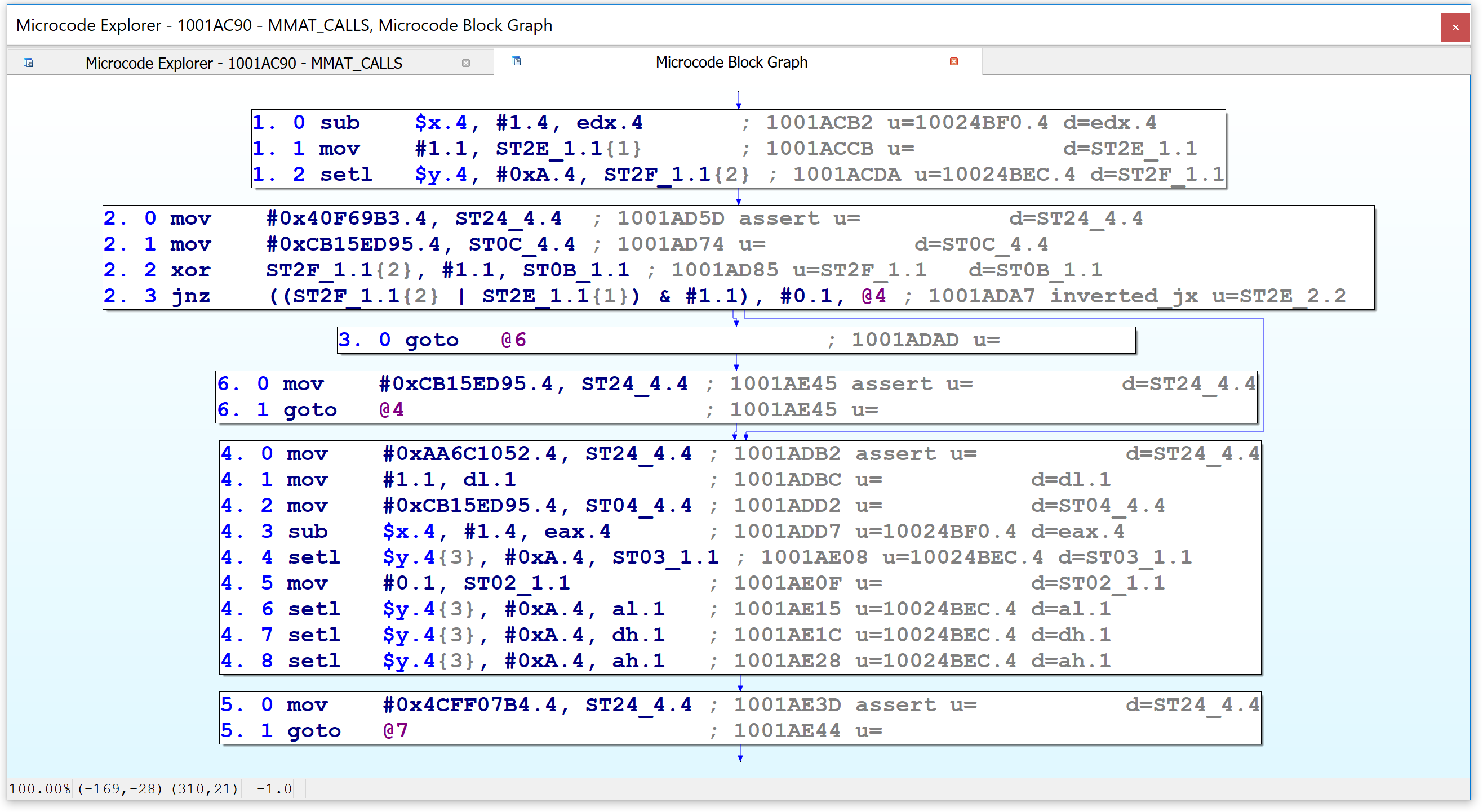
G in the custom viewer will display a graph of the entire microcode representation. For example:
Second, the Microcode Explorer can display the graph for a selected microinstruction and its operands, akin to the VDS5
plugin we saw earlier which displayed a graph of a function’s CTREE representation. Simply position your cursor on any
line in the viewer and press the I key.
The appendix discusses the microcode instruction set in more detail, and I recommend that aspiring microcode API plugin developers read it.
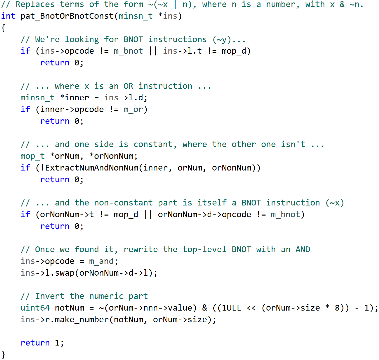
Pattern Deobfuscation with the Microcode API
Once I had a basic handle on the microcode API instruction set, I began by porting my CTREE-level pattern matching and replacement code to the microcode API. This was more laborious due to the more elaborate nature of the microcode API, and the fact I had to write it in C++ instead of Python. All in all, the porting process was mostly straightforward. The code can be found here, and here’s an example of a pattern match and replacement.
Also, I needed to know how to integrate my pattern replacement with the rest of Hex-Rays’ decompiler infrastructure. It
was easy enough to write and test my pattern replacement code against the data returned by the
gen_microcode() API, but doing so has no effect on the decompilation listing that the user ultimately
sees (since the decompiler calls gen_microcode() internally, and we don’t have access to the mbl_array_t
that it generates).
The VDS10 SDK sample illustrates how to integrate pattern-replacement into the Hex-Rays infrastructure. In particular,
the SDK defines an “instruction optimizer” data type called optinsn_t. The virtual method optinsn_t::func()
is given a microinstruction as input. That method must inspect the provided microinstruction and try to optimize it,
returning a non-zero value if it can. Once the user installs their instruction optimizer with the SDK function install_optinsn_handler(),
their custom optimizer will be called periodically by the Hex-Rays decompiler kernel, thus achieving integration that
ultimately affects the user’s view of the decompilation listing.
You may recall that a major impetus for moving the pattern-matching to the microcode world was that, after the replacements had been performed, Hex-Rays had an opportunity to improve the code further via standard compiler optimizations. We showed what we expected the result of such optimizations would be, but no optimizations had been applied when we wrote our pattern-replacement with the CTREE API. By moving to the microcode world, now we do get the compiler optimizations we desire.
After installing our pattern-replacement hook, here’s the decompilation listing for the compiler optimization animation shown earlier:
That’s exactly the result we had been expecting. Great! I didn’t have to code those optimizations myself after all.
Aside: Tricky Issues with Pattern Replacement in the Microcode World
When we wrote our CTREE pattern matching and replacement code, we targeted a specific CTREE maturity level, which lead to predictable CTREE data structures implementing the patterns. In the microcode world, as discussed more in the appendix, the microcode implementation changes dramatically as it matures. Furthermore, our instruction optimizer callback gets called all throughout the maturity lifecycle. Some of our patterns won’t yet be ready to match at earlier maturity phases; we’ll have to write our patterns targeting the lowest maturity level at which we can reasonably match them.
While porting my CTREE pattern replacement code to the microcode world, at first I also adopted my strategy from the
CTREE world of generating my pattern replacement objects from scratch, and inserting them into the microcode atop the
terms I wanted to replace. However, I experienced a lot of difficulty in doing so. Since I was new to the microcode API,
I did not have a clear mental picture of what Hex-Rays internally expected about my microcode objects, which lead to
mistakes (internal errors and a few crashes). I quickly switched strategies such that my replacements would modify the
existing microinstruction and microoperand objects, rather than generating my own, which reduced my burden of generating
correct minsn_t and mop_t objects (since this strategy allowed me to start from valid
objects).
Control Flow Unflattening, Overview
To recap, control flow flattening eliminates direct block-to-block control flow transfers. The flattening process introduced a “block number variable” which determines the block that should execute at each step of the function’s execution. Each flattened function’s control flow structure has been changed into a switch over the block number variable, which ultimately shepherds execution to the correct block. Every block must update the block number variable to indicate the block that should execute next after the current one (where conditional branches are implemented via conditional move instructions, updating the block number variable to the block number of either the taken branch, or of the non-taken branch).
The control flow unflattening process is conceptually simple. Put simply, our task is to rebuild the direct
block-to-block control flows, and in so doing, eliminate the control flow switch mechanism. Implementation-wise,
unflattening is integrated with the Hex-Rays decompiler kernel in a similar fashion to how we integrated
pattern-matching. Specifically, we register an optblock_t callback object with Hex-Rays, such that our
unflattener will be automatically invoked by the Hex-Rays kernel, providing a fully automated experience for the user.
The next chapter will discuss the implementation in more depth.
In the following subsections, we’ll show an overview of the process pictorially. Just three steps are all we need to remove the control flow flattening. Once we rebuild the original control flow transfers, all of Hex-Rays’ existing machinery for control flow restructuring will do the rest of the work for us. This was perhaps my favorite result from this project; all I had to do was re-insert proper control flow transfers, and Hex-Rays did everything else for me automatically.
Step #1: Determine Flattened Block Number to Hex-Rays Block Number Mapping
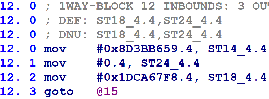
Our first task is to determine which flattened block number corresponds to which Hex-Rays mblock_t. The
following figure is the microcode-level representation for a small function’s control flow switch:
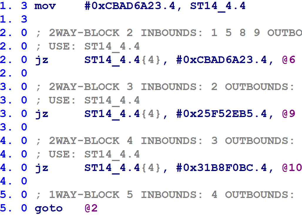
Hex-Rays is currently calling the block number variable ST14_4.4. If that variable matches
0xCBAD6A23,
the jz instruction on block @2 transfers control to block @6. Similarly, 0x25F52EB5
corresponds to block @9, and 0x31B8F0BC corresponds to block @10. The information just described is the
mapping between flattened block numbers and Hex-Rays block numbers. (Of course, our plugin will need to extract it
automatically.)
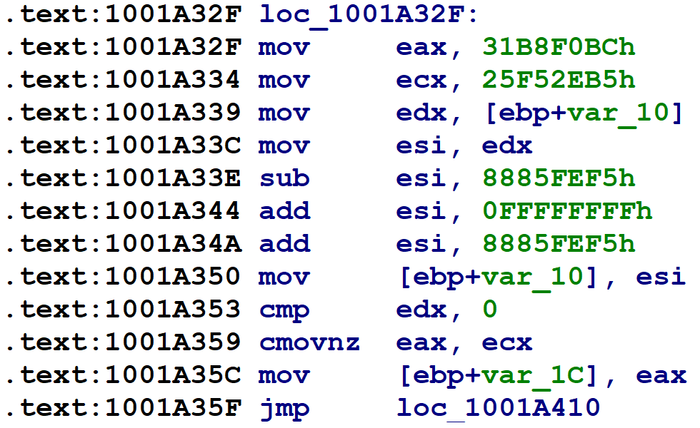
Step #2: Determine Each Flattened Block’s Successors
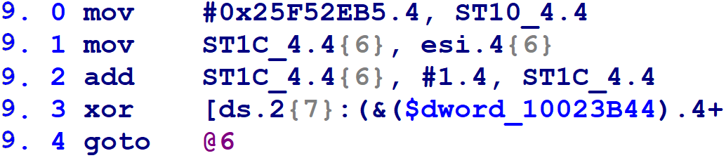
Next, for each flattened block, we need to determine the flattened block numbers to which it might transfer control. Flattened blocks may have one successor if their original control flow was unconditional, or two potential successors if their original control flow was conditional. First, here’s the microcode from block @9, which has one successor. (Line 9.3 has been truncated because it was long and its details are immaterial.)
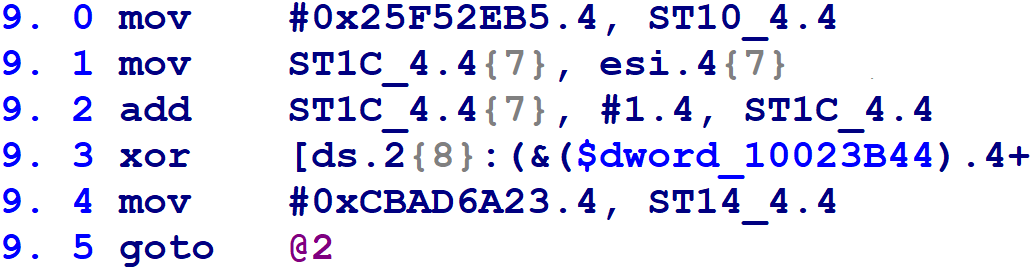
We can see on line 9.4 that this block updates the block number variable to 0xCBAD6A23, before executing
a goto back to the control flow switch (on the Hex-Rays block numbered @2). From what we learned in step
#1, we know that, by setting the block number variable to this value, the next trip through the control flow switch will
execute the Hex-Rays mblock_t numbered @6.
The second case is when a block has two possible successors, as does Hex-Rays block @6 in the following figure.
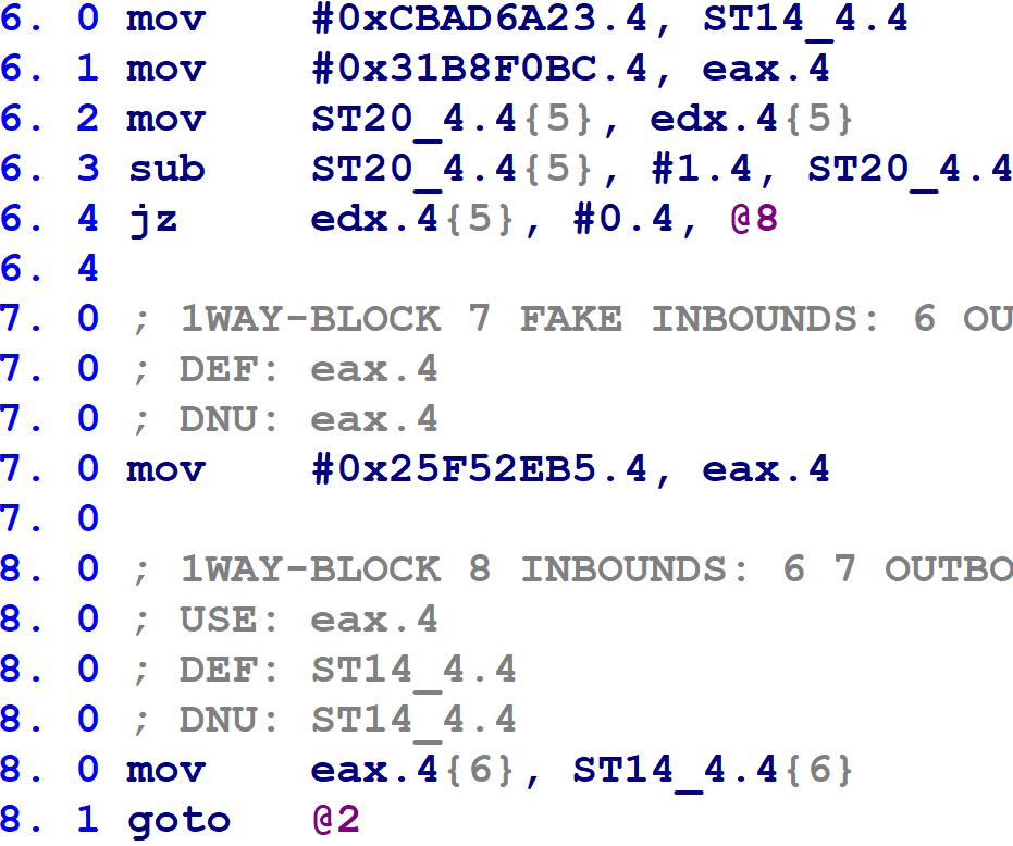
Line 8.0 updates the block number variable with the value of eax, before line 8.1 executes a
goto back to the control flow switch at Hex-Rays block @2. If the jz instruction on line
6.4 is taken, then eax will have the value 0x31B8F0BC (obtained on line 6.1). If the
jz instruction is not taken, then eax will contain the value 0x25F52EB5
from the assignment on line 7.0. Consulting the information we obtained in step #1, this block will transfer control to
Hex-Rays block @10 or @9 during the next trip through the control flow switch.
Step #3: Insert Control Transfers Directly from Source Blocks to Destinations
Finally, now that we know the Hex-Rays mblock_t numbers to which each flattened block shall pass control,
we can modify the control flow instructions in the microcode to point directly to their successors, rather than going
through the control flow switch. If we do this for all flattened blocks, then the control flow switch will no longer be
reachable, and we can delete it, leaving only the function’s original, unflattened control flow.
Continuing the example from above, in the analysis in step #2, we determined that Hex-Rays block @9 ultimately
transferred control to Hex-Rays block @6. Block @9 ended with a goto statement back to the control flow
switch located on block @2. We simply modify the target of the existing goto statement to point to block
@6 instead of block @2, as in the following figure. (Note that we also deleted the assignment to the block number
variable, since it’s no longer necessary.)
The case where a block has two potential successors is slightly more complicated, but the basic idea is the same: altering the existing control flow back to the control flow switch to point directly to the Hex-Rays targeted blocks. Here’s Hex-Rays block @6 again, with two possible successors.
To unflatten this, we will:
- Copy the instructions from block @8 onto the end of block @7.
- Change the
gotoinstruction on block @7 (which was just copied from block @8) to point to block @9 (since we learned in step #1 that0x25F52EB5corresponds to block @9). - Update the
gototarget on block @8 to block @10 (since we learned in step #1 that0x31B8F0BCcorresponds to block @10).
We can also eliminate the update to the block number variable on line 8.0, and the assignments to eax on
lines 6.1 and 7.0.
That’s it! As we make these changes for every basic block targeted by the control flow switch, the control flow switch dispatcher will lose all of its incoming references, at which point we can prune it from the Hex-Rays microcode graph, and then the flattening will be gone for good.
Control Flow Unflattening, In More Detail
As always, the real world is messier than curated examples. The remainder of this section details the practical engineering considerations that go into implementing unflattening as a fully-automated procedure.
Heuristically Identifying Flattened Functions
It turns out that a few non-library functions within the binary were not flattened. I had enough work to do simply making my unflattening code work for flattened functions, such that I did not need the added hassle of tracking down issues stemming from spurious attempts to unflatten non-flattened functions.
Thus, I devised a heuristic for determining whether or not a given function was flattened. I basically just asked myself which identifying characteristics the flattened functions have. I looked at the microcode for a control flow switch:
Two points came to mind:
- The functions compare one variable — the block number variable — against numeric constants in
jzandjginstructions - Those numeric constants are highly entropic, appearing to have been pseudorandomly generated
With that characterization, the algorithm for heuristically determining whether a function was flattened practically wrote itself.
- Iterate through all microinstructions within a function. For this, the SDK handily provides the
mbl_array_t::for_all_topinsnsfunction, to be used with a class calledminsn_visitor_t. - For every
jzandjginstruction that compares a variable to a number, record that information in a list. - After iteration, choose the variable that had been compared against the largest number of constants.
- Perform an entropy check on the constants. In particular, count the number of bits set and divide by the total number of bits. If roughly 50% of the bits were set, decide that the function has been flattened.
You can see the implementation in the code — specifically the
JZInfo::ShouldBlacklist() method.
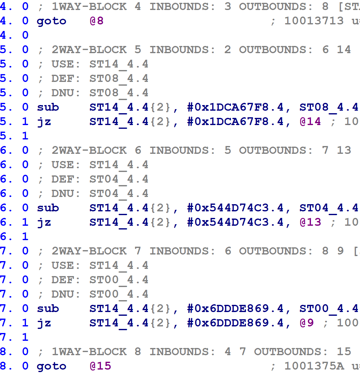
Simplify the Graph Structure
The flattened functions sometimes have jumps leading directly to other jumps, or sometimes the microcode translator
inserts goto instructions that target other goto instructions. For example, in the
following figure, block 4 contains a single goto instruction to block 8, which in turn has a
goto instruction to block 15.
These complicate our later book-keeping, so I decided to eliminate goto-to-goto transfers.
I.e. if block @X ends with a goto @N instruction, and block @N contains a single goto @M
instruction, update the goto @N to goto @M. In fact, we apply this process recursively; if
block @M contained a single goto @P, then we would update goto @N to goto
@P, and so on for any number of chained gotos.
The Hex-Rays SDK sample VDS11 does what was just described in the last paragraph. My code is similar, but a bit more general, and therefore a bit more
complicated. It also handles the case where a block falls through to a block with a single goto — in
this case, it inserts a new goto onto the end of the leading block, with the same destination as the
original goto instruction in the trailing block.
Extract Block Number Information
In step #1 of the unflattening procedure described previously, we need to know:
- Which variable contains the block number
- Which block number corresponds to which Hex-Rays microcode block
When heuristically determining whether a function appears to have been flattened, we already found the variable with the most conditional comparisons, and the numbers it was compared against. Are we done? No — because as usual, there are complications. Many of the flattened functions use two variables, not one, for block number-related purposes. For those that use two, the function’s basic blocks update a different variable than the one that is compared by the control flow switch construct. I call this the block update variable. and I renamed my terminology for the other one to the block comparison variable. Toward the beginning of the control flow switch, the value of the block update variable is copied into the block comparison variable, after which all subsequent comparisons reference the block comparison variable. For example, see the following figure:
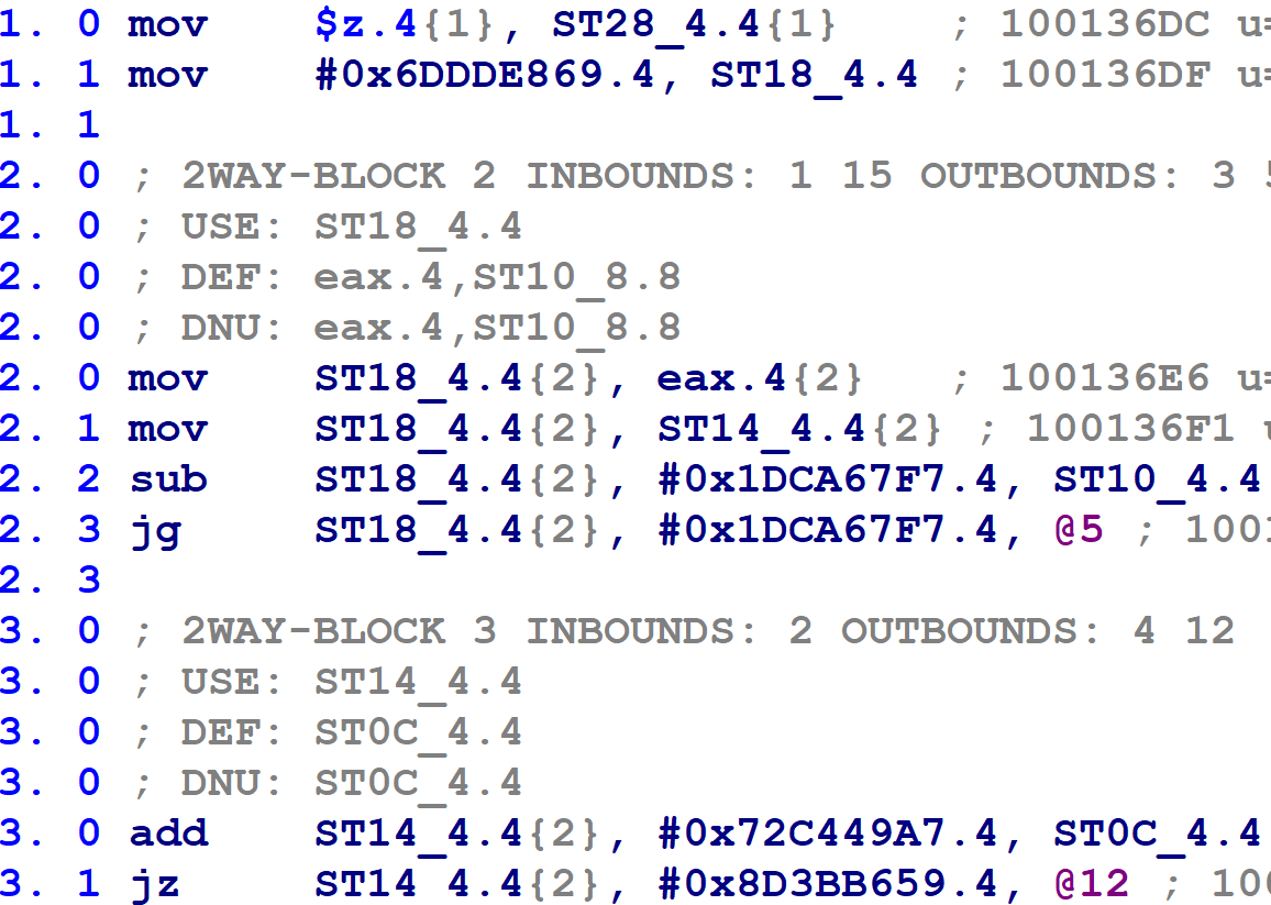
In the above, block @1 is the function’s prologue. The control flow switch begins on block @2. Notice that block @1
assigns a numeric value to a variable called ST18_4.4. Note that the first comparison in the control flow
switch, on line 2.3, compares against this variable. Note also that line 2.1 copies that variable into another variable
called ST14_4.4, which is then used for the subsequent comparisons (as on line 3.1, and all control flow
switch comparisons thereafter).
Then, the function’s flattened blocks update the variable ST18_4:
(Confusingly, the function’s flattened blocks update both variables — however, only the assignment to the block update
variable ST18_4.4 is used. The block comparison variable, ST14_4.4, is redefined on line
2.1 above before its value is used.)
So, we actually have three tasks:
- Determine which variable is the block comparison variable (which we already have from the entropy check).
- Determine if there is a block update variable, and if so, which variable it is.
- Extract the numeric constants from the
jzcomparisons against the block comparison variable to determine the flattened block number to Hex-Raysmblock_tnumber mapping.
I quickly examined all of the flattened functions to see if I could find a pattern as to how to locate the block update variable. It was simple enough: for any variable assigned a numeric constant value in the first block, see if it is later copied into the block comparison variable. There should be only one of these. It was easy to code using similar techniques to the entropy check, and it worked reliably.
The code for reconstructing the flattened Hex-Rays block number mapping is nearly identical to the code used for heuristically identifying flattened functions, and so we don’t need to say anything in particular about it.
Unflattening
From the above, we now know which variable is the block update variable (or block comparison variable, if there is
none). We also know which flattened block number corresponds to which Hex-Rays mblock_t number.
For every flattened block, we need to determine the number to which it sets the block update variable. We walk
backwards, from the end of the flattened block region, looking for assignments to the block update variable. If we find
an assignment from another variable, we recursively begin tracking the other variable. If we find a number, we’re done.
As described previously, flattened blocks come in two cases:
- The flattened block always sets the block update variable to a single value (corresponding to an unconditional branch).
- The flattened block uses an x86
CMOVinstruction to set the block update variable to one of two possible values (corresponding to a conditional branch).
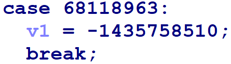
In the first case, our job is simply to find one number. For example, the following flattened block falls into case #1 from above:
In this case, the block update variable is ST14_4.4. Our task is to find the numeric assignment on line
9.4. In concert with the flattened block number Hex-Rays mblock_t number mapping we extracted from the
previous step, we can now change the goto on the final line to the proper Hex-Rays
mblock_t number.
The following flattened block falls into the second case:
Our job is to determine that ST14_4.4 might be updated to either 0xCBAD6A23 or 0x25F52EB5
on lines 6.0 and 7.0, respectively.
Complication: Flattened Blocks Might Contain Many Hex-Rays Blocks
This part of the project forced me to contend with a number of complications, some of which aren’t shown by the examples above.
One complication is that a flattened block may be implemented by more than one Hex-Rays mblock_t as in
the first case above, or more than three Hex-Rays mblock_t objects in the second case above. In
particular, Hex-Rays splits basic blocks on function call boundaries — so there may be any number of Hex-Rays mblock_t
objects for a single flattened block. Since we need to work backwards from the end of a flattened region, how do we know
where the end of the region is? I solved this problem by computing the function’s dominator
tree
and finding the block dominated by the flattened block header that branches back to the control flow switch.
Complication: Data-Flow Tracking
Finding the numeric values assigned to the block update variable ranges from trivial to “mathematically hard”. I wound up cheating in the mathematically hard cases.
Sometimes Hex-Rays’ constant propagation algorithms make our lives easy by creating a microinstruction that directly moves a numeric constant into the block update variable. A slightly less simple, but still easy, case is when the assignment to the block update variable involves a number being copied between a few registers or stack variables along the way. As long as there aren’t any errant memory writes to clobber saved values on the stack, it’s easy enough to follow the chain of mov instructions backwards back to the original constant value.
To handle both of these cases, I wrote a function that starts at the bottom of a block and searches for assignments to the block number variable in the backwards direction. For assignments from other variables, it resumes searching for assignments to those variables. Once it finally finds a numeric assignment, it succeeds.
However, there is a harder case for which the above algorithm will not work. In particular, it will not work when the flattened blocks perform memory writes through pointers, for which Hex-Rays cannot determine legal pointer value sets. Hex-Rays, quite reasonably, can not and does not perform constant propagation across memory values if there are unknown writes to memory in the meantime. Such transformations would break the decompilation listing and cause the analyst not to trust the tool. And yet, this part of the project presents us with the very problem of constant propagation across unknown memory writes.
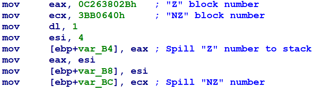
Here’s an example of the hard case manifesting itself. At the beginning of a flattened block, we see the two destination block numbers being written into registers, and then saved to stack variables.
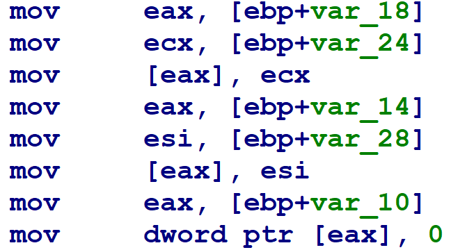
Later on, the flattened block has several memory writes through pointers.
Finally, at the end of the block, the destination block numbers — which were spilled to stack variables at the beginning of the flattened block — are then loaded from their stack slots, and used in a conditional block number update.
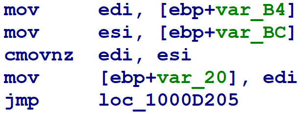
The problem this presents us is that we need, or Hex-Rays needs, to formally prove that the memory writes in the middle
did not overwrite the saved block update numbers. In general, pointer aliasing is an undecidable problem, meaning it is
impossible to write an algorithm to solve every instance of it.
So instead, I cheated. When my numeric definition scanner encounters an instruction whose memory side effects cannot be
bounded, I go to the beginning of the flattened block region and scan forwards looking for numeric assignments to the
last variables I was tracking before encountering an unbounded memory reference. I.e., in the three assembly snippets
above, I jump to the first one and find the numeric assignments to var_B4 and var_BC.
This is a hack; it’s unsafe, and could very well break. But, it happens to work for every function in this sample, and
will likely work for every sample compiled by this obfuscating compiler.
Appendix: More about the Microcode API
What follows are some topics about the Microcode API that I thought were important enough to write up, but I did not want them to alter the narrative flow. Perhaps you can put off reading this appendix until you get around to writing your first microcode plugin.
The Microcode Verifier
Chances are good that if you’re going use the microcode API, you probably will be modifying the microcode objects described in the previous section. This is murky territory for third-party plugin developers, especially those of us who are new to the microcode API, since modifying the microcode objects in an illegal fashion can lead to crashes or internal errors.
To aid plugin developers in diagnosing and debugging issues stemming from illegal modifications, the microcode API
offers “verification”, which is accessible in the API through a method called mbl_array_t::verify(). (The
other objects also support verification, but their individual verify() methods are not currently exposed
through the API.) Basically, mbl_array_t::verify() applies a comprehensive set of test suites to the
microcode objects (such as mblock_t, minsn_t, and mop_t).
For one example of verification, Hex-Rays has a set of assumptions about the legal operand types for its
microinstructions. The m_add instruction must have at least two operands, and those operands must be the same size.
m_add can optionally store the result in a “destination” operand; if this is the case, certain destination types are
illegal (e.g., in C, it does not make any sense to have a number on the left-hand side of an assignment statement, as in
1 = x + y;. The analogous concept in the microcode world, storing the result of an addition into a
number, also does not make sense and should be rejected as illegal.)
The source code for the verify() methods is included in the Hex-Rays SDK under
verifier\verify.cpp. (There is an analogous version for the CTREE API under
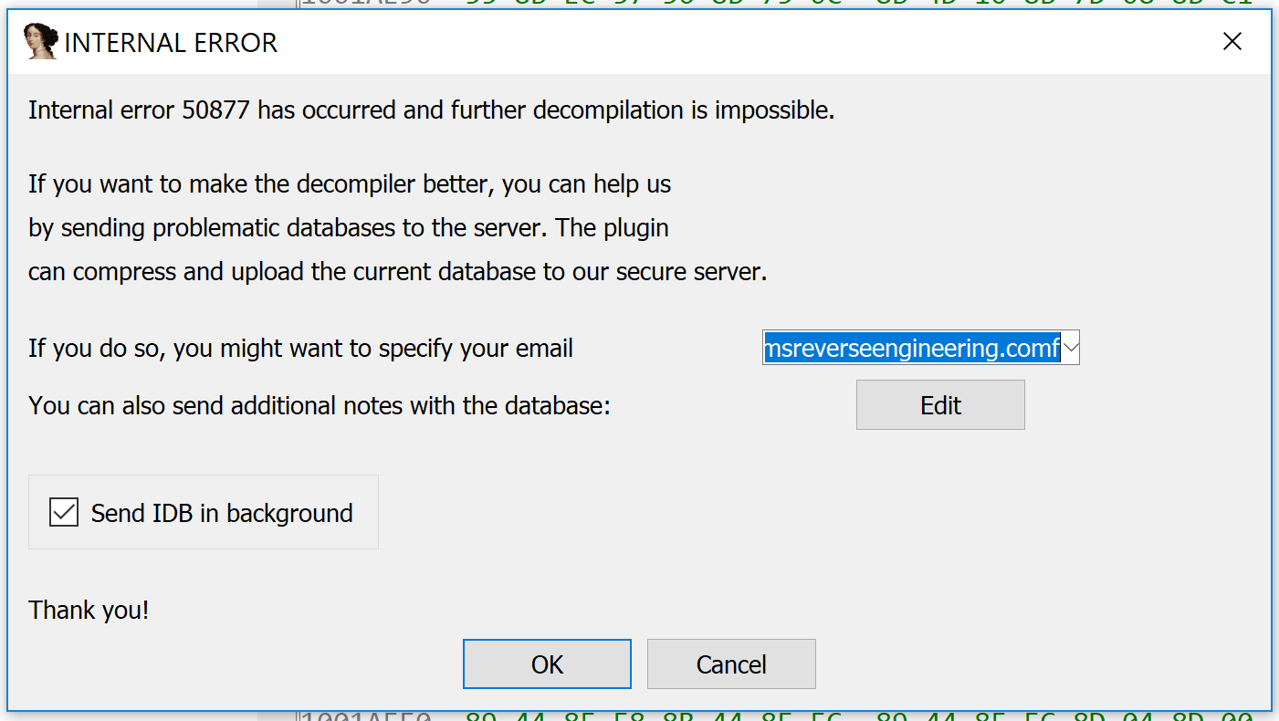
verifier\cverify.cpp.) When the verifier detects an illegal condition, it raises a numbered “internal
error” within IDA, as in the following screenshot. The plugin developer can search for this number within the verifier
source code to determine the source of the error.
The verifier source code is, in my opinion, the best and most important source of documentation about Hex-Rays’ internal expectations. It touches on many different parts of the microcode API, and provides examples of how to call certain API functions that may not be covered by the other example plugins in the SDK. Wading through internal errors, tracking them down in the verifier, and learning Hex-Rays’ expectations about the microcode objects (as well as how it verifies them) is a rite of passage for any would-be microcode API plugin developer.
Intermediate Representations and the Microcode Instruction Set
If you’ve ever studied compilers, you are surely familiar with the notion of an intermediate representation. The minsn_t
and mop_t data types, taken together, are the intermediate represention used in the microcode phase of
the Hex-Rays decompiler.
If you’ve studied compilers at an advanced level, you might be familiar with the idea that compilers frequently use more
than one intermediate representation. For example, Muchnick describes a compiler archetype using three intermediate
representations, that he respectively calls HIR (“high-level” intermediate representation), MIR (“mid-level”), and LIR
(“low-level”).
HIR resembles a high-level language such as C, which supports nested expressions. I.e., in C, one may perform multiple
operations in a single statement, such as a = ((b + c) * d) / e. On the other hand, low-level languages
such as LIR or assembly generally can only perform one operation per statement; to represent the same code in a
low-level language, we would need at least three statements (ADD, MUL, and DIV). LIR is basically a “pseudo-assembly
language”.
So then, given that the Hex-Rays microcode API has only intermediate representation, which type is it — is it closer to HIR, or is it closer to LIR? The answer is, it uses a clever design to simulate both HIR and LIR! As the microcode matures, it is gradually transformed from a LIR-like representation, with only one operation per statement, to a HIR-like representation, with arbitrarily many operations per statement. Let’s take a closer look with the microcode explorer.
When first generating the microcode (i.e., microcode maturity level MMAT_GENERATED), we can see that the
microcode looks a lot like an assembly language. Notice that each microinstruction has two or three operands apiece, and
each operand is something like a number, register name, or name of a global variable. I.e., this is what we would call
LIR in a compiler back-end.
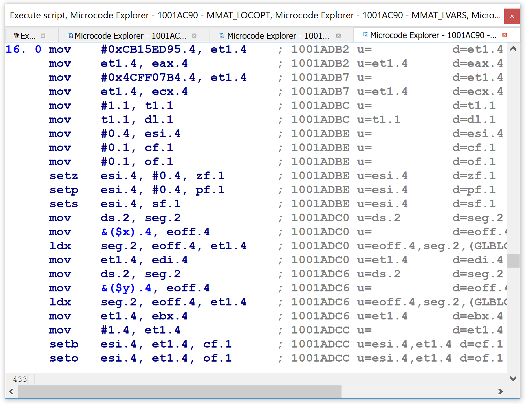
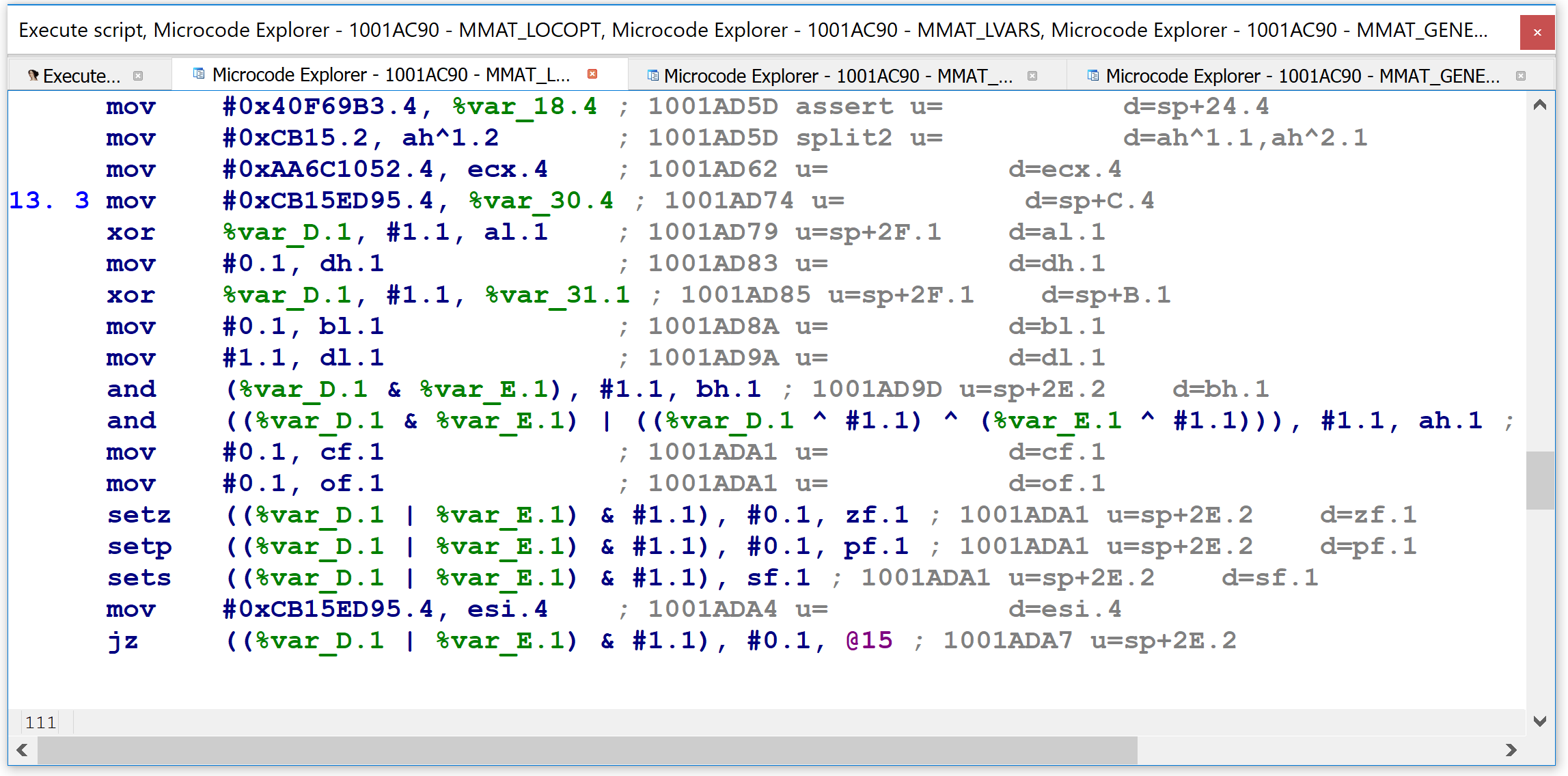
Shortly thereafter in the maturity pipeline, in the MMAT_LOCOPT phase, we can see that the microcode
representation for the same code in the same function is already quite different. In the figure below, many of the lines
in the bottom half have complex expressions inside them, instead of the simple operands we saw just previously. I.e., we
are no longer dealing with LIR.
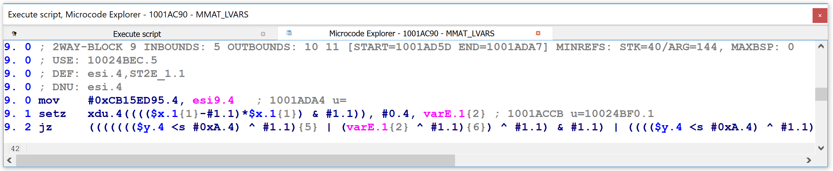
Finally, at the highest level of microcode maturity, MMAT_LVARS, the same code has shrunk down to three
lines, with the final one being so long that I had to truncate it to fit it reasonably into the picture:
Microinstructions and Microoperands
That’s a pretty impressive trick — supporting multiple varieties of compiler IRs with a single set of data types. How did they do it? Let’s look more carefully at the internal representations of microinstructions and microoperands to figure it out.
Respectively, microinstructions and microoperands are implemented via the minsn_t and
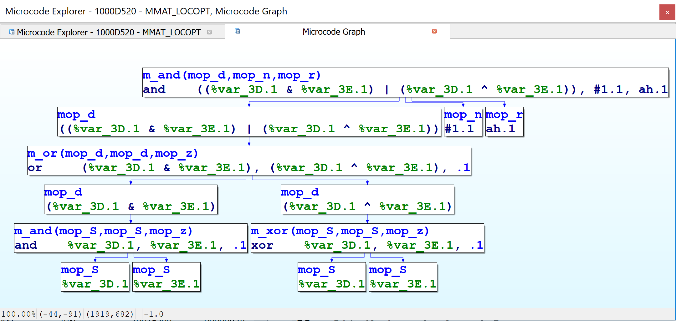
mop_t classes. Here again is the graph representation for a microinstruction:
In the figure above, the top-level microcode instruction is shown in the topmost node. It is represented by an
instruction of type m_and, which in this case uses three comma-separated operands, of type
mop_d (result of another instruction), mop_n (a number), and mop_r
(destination is a register). The mop_d operand is a compound instruction with two expressions joined
together with a bitwise OR — thus, it corresponds to a microinstruction of type m_or, whose operands
themselves are respectively the result of bitwise AND and bitwise XOR operands, and as such, these operands are of type
mop_d, instructions respectively of type m_and and m_xor. The inputs to the
AND and XOR operators are all stack variables, i.e., micro-operands of type mop_S.
Now we can see how the microcode API supports such dramatic differences in microcode representation using the same
underlying data structures. Specifically, the example above makes use of the mop_d microoperand type,
which refers to the result of another microinstruction. I.e., microinstructions contain microoperands, and microoperands
can contain microinstructions (which then contain other microoperands, which may recursively contain other
microinstructions, etc). This technique allows the same data structures to represent both HIR- and LIR-like
representations. The initial microcode generation phase does not generate mop_d operands. Subsequent
maturity transformations introduce them in order to build a higher-level representation.
The proper name for this language design technique is mutual recursion: where one category of a grammar refers to another category, and the second refers back to the first. I found this design technique very elegant and clever. Apart from using different data structures at each level of representation, I can’t think of any cleaner ways to accommodate multi-level representations. That said, this type of programming is mostly common only among people with serious professional experience with programming language theory and compiler internals. Ordinary developers would do well to study some programming language theory if they want to make good use of the microcode API.